


Goal
The notebook behind this post implements the following paper from 2011 with around 20 citations, How Much Is Enough? Choosing Epsilon for Differential Privacy by Jaewoo Lee et al.
Paper summary
Even though Differential Privacy (DP) in principle protects any individual in a dataset by cloaking with noise the result of an analytics query, DP has its limitations. The limitation addressed in this paper is based on the finite amount of dataset possibilities that a worst-case adversary model (Almost perfect background knowledge and infinite computation power) considers after seeing the output of the DP query. Because some actual dataset distributions are more likely than others, the adversary can update his/her knowledge more efficiently. Therefore, this imbalance needs to be taken into consideration when calculating epsilon. The authors formulated a tight bound for epsilon with binary search based on disclosure risk, which acknowledges this DP defect.
Opinion on the paper
My humble opinion is that the paper is concise, elegant, and can take your understanding of DP further. I would like to thank the authors Jaewoo Lee and Chris Clifton for these days I spent implementing :) Moreover, I invite everyone to look at the paper and check the code to understand it better.
Jump to the replicated figures if you are impatient :)
The notebook allows you to expand and test the paper's approach for different queries. They plot the mean query, but I also plotted the median query. I encourage you to get my code and plot, e.g., the variance query.
Notebook contributions
- I coded a function that calculates the bounded and unbounded sensitivity of a dataset containing numeric columns. However, how to code the algorithm was not explained in the paper. With these functions, you can also vary the Hamming distance k (Check these functions in this blog post). How does it do it? Empirically - This function creates all possible neighboring datasets with k less or more records for unbounded DP and with the same amount of records but changing k values for bounded DP. Once the function creates the neighboring datasets, it calculates the sensitivity empirically. More specifically, the function calculates the query result for each possible neighboring dataset, calculates all possible L1 norms, and then chooses the maximum. Note that, for simplicity's sake for unbounded DP, the function selects the largest sensitivity between the two paradigms: one more record or one less record.
- I found no mistakes in the paper, only a typo in a number in a formula. The numerator should be 0.3062 and not 0.3602 on page 333 (Page 9 of the PDF).
- I coded the formulas for a uniform prior, posterior, upper, and tighter bound of the posterior for any given dataset and a set of query types.
- I coded the binary search explained in the paper to find the correct epsilon value (Given a disclosure risk) for any query type.
- With this code, you can easily play around by using larger or different datasets than the one used in the paper. I used the exact data from the paper to replicate the results.
- This notebook implements more queries beyond the mean and the median used for explanations in the paper. I encourage you to try them out!
IMPORTANT: The authors use an approximation of sensitivity Δv (Section 5.1 Equations 4,5) based on the released dataset and its neighbors. Furthermore, they use sensitivity based on unbounded DP (Δf) to calculate the upper bound. In this notebook, however, I use the definition for sensitivity based on bounded DP as Δv. I do this because, to the best of my knowledge, bounded DP sensitivity should be equal to the one the authors chose as long as I keep the Hamming distance to 1. However, given that the results obtained are the same as the authors, we can be sure that my approach is correct. Perhaps back then, the terms bounded and unbounded DP were not commonly used. Therefore, the beautiful unmentioned contribution of this paper is that the authors use bounded and unbounded sensitiviy to calculate the correct value of epsilon.
Some concepts before we start:
- When I talk about bounded sensitivity, I refer to the sensitivity that comes from a bounded DP definition, i.e., the neighboring dataset is built by changing the dataset's records (Not adding or removing records). E.g., with x = {1, 2, 3} from universe X = {1, 2, 3, 4}, a neighboring dataset in this case would be: x' = {1, 2, 4}
- When I talk about unbounded sensitivity, I refer to the sensitivity that comes from an unbounded DP definition, i.e., the neighboring dataset is built by adding or removing records. E.g., with x = {1, 2, 3} and universe X = {1, 2, 3, 4}, a neighboring dataset in this case could be: x' = {1, 2} or {1, 3} or {1, 2, 3, 4}
- The prior is the prior knowledge of an adversary, i.e., his/her best guess about which dataset is probably the real one. The paper and this notebook assume a uniform prior.
- The posterior is the updated knowledge of the adversary, i.e., once he/she has seen the query results, the posterior maps a probability to a possible real dataset. The higher it is, the more confident will the adversary be about a dataset being the real one.
Note: The author uses "Pr" to denote cumulative distribution functions and "P" to refer to probability density functions. So when you see P(k(w) = x), it is not the point mass at x; instead, the authors refer to the value of the probability density at x. "P" is used in Definition 3 onwards. However, for section 4.1, the author used the cumulative distribution function, using "Pr." For Definition 3, he could have used the cumulative distribution function; qualitatively, the result would be the same. Most importantly, this notation (P(k(w) = x)) is also used in section 5.1.
Results
This is the plot I replicated faithfully from the paper:
I applied a binary search and found the optimal values for epsilon. Have a look:
I went a step further and also plotted the median and found the optimal values for epsilon. Here is the result:
Notebook
The notebook is too large to share fully here; therefore, I will take the most important snippets and discuss them instead. For the rest of the notebook, I invite you to find the full version in GitHub. Furthermore, we will only cover here the most relevant functions to implement this paper, other cool functions like calculating the sensitivity empirically will be shown in future blog posts. Furthermore, if you want to check how I could successfully calculate every calculation output from the paper, then you are invited to follow along the notebook.
We will use the following dataset to define the universe of possible values throughout the notebook to test the paper, it contains the setting's universe values from the people the author's of the paper want to protect. To simplify things without the loss of generality, the authors just use 4 people. The 4 people belong to a high school. The high school would like to release a dataset to be queried; however, this new dataset will not include people that have been on probation, in this case, Terry.
# We define the actual dataset (conforming the universe)
dict_school = {'name': ['Chris', 'Kelly', 'Pat', 'Terry'], 'school_year': [1, 2, 3, 4], 'absence_days': [1, 2, 3, 10]}

df_school = pd.DataFrame(dict_school)
df_school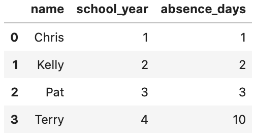
The attacker's ultimate goal is to find out which student was placed on probation, Terry. However, the attacker will only be able to query this other dataset below (The release dataset does not contain Terry, because the release dataset only contains students who were not in probation):
# We define the the dataset that we will release
df_school_release = df_school.drop([3], axis=0)
df_school_release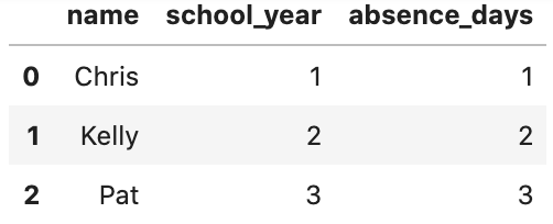
To accomplish this, the attacker would perform analytics queries on df_school_release such as the mean. With the results, the adversary will try to improve his/her guess about which dataset is the true one to single out and discover the student who was placed on probation (Terry).
In summary, the adversary model adopted in the paper is the worst-case scenario. It will be the one I adopted in this notebook as well: An attacker has infinite computation power and complete knowledge of the dataset except for one individual (Informed attacker). Because DP is supposed to provide privacy given adversaries with arbitrary background knowledge, it is appropriate to assume that the adversary has full access to all the records (Knows all the universe, i.e., df_school). However, there is a dataset generated from the universe without an individual (df_school_release), and he does not know who is and who is not in this dataset (This is the only thing he does not know). However, he knows this dataset contains people with a certain quality (The students who have not been on probation). With the initial dataset, the attacker will reconstruct the dataset he does not know, querying the new dataset (df_school_release) without access.
As I mentioned, there are more functions in the notebook, however, let us show here the ones that are most relevant for the paper replication.
We assume the attacker has a uniform prior:
def prior_belief(universe, universe_subset, columns):
    """
    INPUT:
        universe - (df) contains all possible values of the dataset
        universe_subset - (df) contains the values of the dataset to be released
        columns - (array) contains the names of the columns we would like to obtain the sensitivity from

    OUTPUT:
        prior_per_column - (dict) maps each column of all the possible release datasets to the prior knowledge of an adversary

    Description:
    It calculates the prior knowledge of an adversary assuming uniform distribution
    """
    # Initialize the dictionary to store all the posteriors with the column names as keys
    prior_per_column = {}

    for column in columns:

        # We calculate all the possible release datasets
        release_datasets = itertools.combinations(universe[column], len(universe_subset[column]))
        release_datasets = list(release_datasets)
        number_possible_release_datasets = len(release_datasets)
        # We assume a uniform prior
        prior_per_column[column] = [1 / number_possible_release_datasets] * number_possible_release_datasets

    return prior_per_column
(Have in mind that I coded these functions to work with larger datasets, so the code may be transferred to other applications)
In this prior, we calculated all possible datasets that the attacker may conceive with the universe. If the universe is of size 4, and the released dataset is of size 3, then the number of possible release datasets is (4 choose 3), which is 4. In this code snippet, I went over the top, creating the actual neighboring datasets with itertools. For the prior is not needed, but I was tinkering a lot when creating the notebook. If the prior is not uniform, then you could assign a probability mass function to the range of possible release datasets.
Coming back to what was previously explained, for clarification: Once the attacker has a random query output from the hidden dataset, the attacker will try to see which one of these 4 worlds is more likely to output the query result.
Now we define the posterior; this is one of the most exciting bits of the notebook. The posterior is the updated knowledge of the attacker once she gets the output from the query. This code snippet below codes Definition 3 (It also appears in equation 2 of Section 5.1 but in another form, right before the triangle inequality). If there is little noise, the posterior will gravitate towards a particular possible dataset; the distribution would go from uniform (the prior) to something skewed towards the actual dataset.
def posterior_belief(universe, universe_subset, columns, query_type, query_result, sensitivity, epsilon):
    """
    INPUT:
        universe - (df) contains all possible values of the dataset
        universe_subset - (df) contains the values of the dataset to be released
        columns - (array) contains the names of the columns we would like to obtain the sensitivity from
        query_type - (str) contain the category declaring the type of query to be later on executed
        query_result - (float) the result of the query the attacker received
        sensitivity - (dict) it maps the columns to their sensitivities, they can be based on bounded or unbounded DP
        epsilon - (float) it is the parameter that tunes noise, based on DP

    OUTPUT:
        posterior_per_column - (dict) maps each column of all the possible release datasets to the posterior knowledge of an adversary

    Description:
    It calculates the posterior knowledge of an adversary
    """


    # Initialize the dictionary to store all the posteriors with the column names as keys
    posterior_per_column = {}

    # We initialie the type of query for which we would like calculate the sensitivity
    query = Query_class(query_type)

    for column in columns:

        # We calculate all the possible release datasets
        release_datasets = itertools.combinations(universe[column], len(universe_subset[column]))
        release_datasets = list(release_datasets)

        # According to the definiton of DP, the sacle factor of a Laplacian distribution:
        scale_parameter = sensitivity[column]/epsilon

        posterior_probability = []
        for release_dataset in release_datasets:
            probability = (1 / (2 * scale_parameter)) * np.exp(- np.abs(query_result - np.mean(release_dataset)) / scale_parameter)
            posterior_probability.append(probability)
            print(probability)
        posterior_per_column[column] = posterior_probability / np.sum(posterior_probability)

    return posterior_per_column
In this function above, the attacker is calculating with the cumulative distribution function (cdf) of the laplace distribution, how likely it is for a dataset to be the actual one given a query output.
The disclosure risk is the highest of the posteriors; if the highest posterior coincides with the true hidden dataset, then the attacker has been successful.
Okay, now we will replicate the upper bound of the adversary's posterior belief (Section 5.1 equation (4)-(5)). This is done to have a theoretical upper bound, which will not necessarily be tight. This however is convenient as you end up with a nice formula for any given circumstance; nonetheless, it will not be tight as we will see (Not being tight is not good :/ because then you might think you need more noise than what you really do, i.e., a lower epsilon than needed).
def upper_bound_posterior(universe, columns, bounded_sensitivity, unbounded_sensitivity, epsilon):
    """
    INPUT:
        universe - (df) contains all possible values of the dataset
        columns - (array) contains the names of the columns we would like to obtain the sensitivity from
        bounded_sensitivity - (dict) it maps the columns to their bounded sensitivities
        unbounded_sensitivity - (dict) it maps the columns to their unbounded sensitivities
        epsilon - (float) it is the parameter that tunes noise, based on DP

    OUTPUT:
        upper_bound_per_column - (dict) dictionary that maps the value that bounds the posterior (also the risk) per column

    Description:
    It calculates the upper bound of the posterior
    """

    upper_bound_posterior_per_column = {}

    for column in columns:

        upper_bound_posterior = 1 / (1 + (universe.shape[0] - 1) * \
                                np.exp(-epsilon * bounded_sensitivity[column] / unbounded_sensitivity[column]))

        upper_bound_posterior_per_column[column] = upper_bound_posterior

    return upper_bound_posterior_per_column
But! We also coded an earlier stage of the formulation of 5.1, so we can get a tighter bound. Down below inequality 3 of Section 5.1 is programmed:
def tighter_upper_bound_posterior(universe, universe_subset, columns, query_type, sensitivity, epsilon, percentile=50):
    """
    INPUT:
        universe - (df) contains all possible values of the dataset
        universe_subset - (df) contains the values of the dataset to be released
        columns - (array) contains the names of the columns we would like to obtain the sensitivity from
        query_type - (str) contain the category declaring the type of query to be later on executed
        sensitivity - (dict) it maps the columns to their sensitivities, they can be based on bounded or unbounded DP
        percentile - (int) percentile value for the percentile query. ONLY VALID IF IT IS THE PERCENTILE QUERY THE ONE BEEN EXECUTED
        epsilon - (float) it is the parameter that tunes noise, based on DP

    OUTPUT:
        tighter_upper_bound_posteriorper_column - (dict) maps each column of all the possible release datasets to
        the tighter upper bound of the posterior knowledge of an adversary

    Description:
    It calculates a tighter bound of the posterior knowledge of an adversary
    """
    # Initialize the dictionary to store all the posteriors with the column names as keys
    tighter_upper_bound_posterior_per_column = {}

    # We initialie the type of query for which we would like calculate the sensitivity
    query = Query_class(query_type)

    for column in columns:

        # We calculate all the possible release datasets
        release_datasets = itertools.combinations(universe[column], len(universe_subset[column]))
        release_datasets = list(release_datasets)


        # We calculate the L1_norm for the different combinations of the query result from different data releass
        # We have to complete all loops becuase we need to calculate different values of the posterior
        # Then we select the max after calculating all posteriors
        posterior_probability = []
        for i in range(0, len(release_datasets) - 1):

            L1_norms = []
            for j in range(0,  len(release_datasets)):

                if release_datasets[i] == release_datasets[j]:

                    continue

                else:

                    L1_norms.append(np.abs(query.run_query(release_datasets[i], percentile) - query.run_query(release_datasets[j], percentile)))

            denominator_posterior = 1
            for L1_norm in L1_norms:

                 denominator_posterior += np.exp(-epsilon * L1_norm / sensitivity[column])

            beta = 1 / denominator_posterior
            posterior_probability.append(beta)

        tighter_upper_bound_posterior_per_column[column] =  max(posterior_probability)

    return tighter_upper_bound_posterior_per_column
Furthermore, we coded the upper bound of epsilon based on inequality 7 of section 5.2. Given a disclosure risk fixed by a practitioner, one may input also the sensitivities (Bounded and unbounded), and the number of possible worlds. However, this value of epsilon is not tight, as it is derived from the upper bound. Unfortunately, one cannot arithmetically get epsilon from the tighter upper bound, that is why the authors suggest to use a binary search, which I did.
Here is the function to calculate the upper bound of epsilon:
def upper_bound_epsilon(universe, columns, bounded_sensitivity, unbounded_sensitivity, risk):
    """
    INPUT:
        universe - (df) contains all possible values of the dataset
        columns - (array) contains the names of the columns we would like to obtain the sensitivity from
        bounded_sensitivity - (dict) it maps the columns to their bounded sensitivities
        unbounded_sensitivity - (dict) it maps the columns to their unbounded sensitivities
        risk - (float) it is a parameter that sets the privacy requirement. It is the probability that the attacker
        succeeds in his/her attack

    OUTPUT:
        epsilon_upper_bound_per_column - (dict) dictionary that maps the upper bound of epsilon per column

    Description:
    It calculates epsilon given a risk willing to take
    """

    epsilon_upper_bound_per_column = {}

    for column in columns:

        epsilon_upper_bound =  unbounded_sensitivity[column] / bounded_sensitivity[column] * \
                            np.log(((universe.shape[0] - 1) * risk) / (1 - risk))
        epsilon_upper_bound_per_column[column] = epsilon_upper_bound

    return epsilon_upper_bound_per_column
After defining our functions, we enter into the MAIN of the notebook. Here I calculate the posterior using the formula for a random query output of 2.2013 (Example output from the paper). The posterior for the first world as you can see on the paper should be 0.6180. (Everything you see from now on is using the mean query)
# Let us calculate the posteriors
query_result = 2.20131
epsilon = 2
query_type = 'mean'
mean_unbounded_global_sensitivities = unbounded_empirical_global_L1_sensitivity(df_school, df_school_release.shape[0], columns,  query_type, hamming_distance)
posteriors = posterior_belief(df_school, df_school_release, columns, query_type, query_result, mean_unbounded_global_sensitivities, epsilon)
posteriors
>>> {'school_year': array([0.33898835, 0.4003158 , 0.17987348, 0.08082237]), 'absence_days': array([0.61802372, 0.15816999, 0.12500781, 0.09879847])}
(Side note: It is because of this output that I can assert there is a typo in the numerator, it should read "0.3062", not "0.3602".)
The output shows the posteriors for each possible world. We see that the maximum posterior for the attribute absence days is 0.6180 as in the paper, which shows that the attacker will think that the real dataset is world 1, which is correct, and, therefore, the attacker was successful. This proves the concern of the authors about choosing epsilon.
# Let us calculate the confidence of the attacker
confidence_adversary = confidence(posteriors, priors, columns)
confidence_adversary
>>> >>> {'school_year': 0.16917763372208006, 'absence_days': 0.15120152863171882}
The function "confidence" takes the maximum posterior and subtracts its probability to the prior to obtain what the authors call "confidence". What this means is that we have updated the beliefs of the attacker by 16.92% for the school year attribute and 15.12% for the absence days attribute.
Now I am going to flex the nice functions we coded in the beginning. In section 5.2 equation 9, the author obtains an epsilon upper bound of around 0.3829 (For this result, the authors consider absence days):
# Let us calculate the upper bound with epsilon with a risk of 0.33 (there is a chance of 1/3 of letting
# the adversary know the true value)
risk = 1/3
epsilon_upper_bound = upper_bound_epsilon(df_school, columns, mean_bounded_global_sensitivities, mean_unbounded_global_sensitivities, risk)
epsilon_upper_bound
>>> {'school_year': 0.3378875900901369, 'absence_days': 0.38293926876882173}
This is the upper bound; however, we can do better choosing a higher epsilon, i.e., choosing a higher epsilon will not push us over the disclosure risk limit of 1/3. In the paper, the result from equation 12 should be 0.3292 (For this result, the authors consider school year)
epsilon = 0.5
query_type = 'mean'
posterior_tighter_upper_bound = tighter_upper_bound_posterior(df_school, df_school_release, columns, query_type, mean_unbounded_global_sensitivities, epsilon)
print('For epsilon {} the posterior is {}'.format(epsilon, posterior_tighter_upper_bound))
>>> For epsilon 0.5 the posterior is {'school_year': 0.3291788293012836, 'absence_days': 0.3476971459619019}
If you are wondering why are we using these upper bounds and not outputting the real value of the posterior instead: In order to plot the real value of the posterior, you already need to have a query result. For someone to output a random query result, he/she had to already decide on a value of epsilon, but this research is about finding the fitting value of epsilon - hence the name of the paper.
The purpose of finding these upper and tighter bounds of the posterior is to find an optimal value for epsilon, i.e., by trying out with many values of epsilon and without knowing which query result the adversary will get, you can still plot the posterior upper and tight bounds and decide which epsilon to pick based on the risk you are willing to take.
Side note: In the paper, they refer to the acceptable risk with the Greek letters delta and rho. Delta is never placed in an equation though, that might be somewhat confusing if you are reading the paper.
Now let us plot these upper and lower bounds. We first need to get the values for the plotting:
precision = 0.01
limit_x = 5
epsilons = np.linspace(0, 5, num=int(limit_x/precision))

# Setting parameters
columns = ['school_year', 'absence_days']
query_type = 'mean'
# Initialize dicts with correspondng keys: https://stackoverflow.com/questions/11509721/how-do-i-initialize-a-dictionary-of-empty-lists-in-python
posterior_upper_bound = {k: [] for k in columns}
posterior_tighter_upper_bound = {k: [] for k in columns}

# Obtaining the values for the bounds
for epsilon in epsilons:

    temp_posterior_upper_bound = upper_bound_posterior(df_school, columns, mean_bounded_global_sensitivities, mean_unbounded_global_sensitivities, epsilon)
    temp_posterior_tighter_upper_bound = tighter_upper_bound_posterior(df_school, df_school_release, columns, query_type, mean_unbounded_global_sensitivities, epsilon)

    for column in columns:

        posterior_upper_bound[column].append(temp_posterior_upper_bound[column])
        posterior_tighter_upper_bound[column].append(temp_posterior_tighter_upper_bound[column])
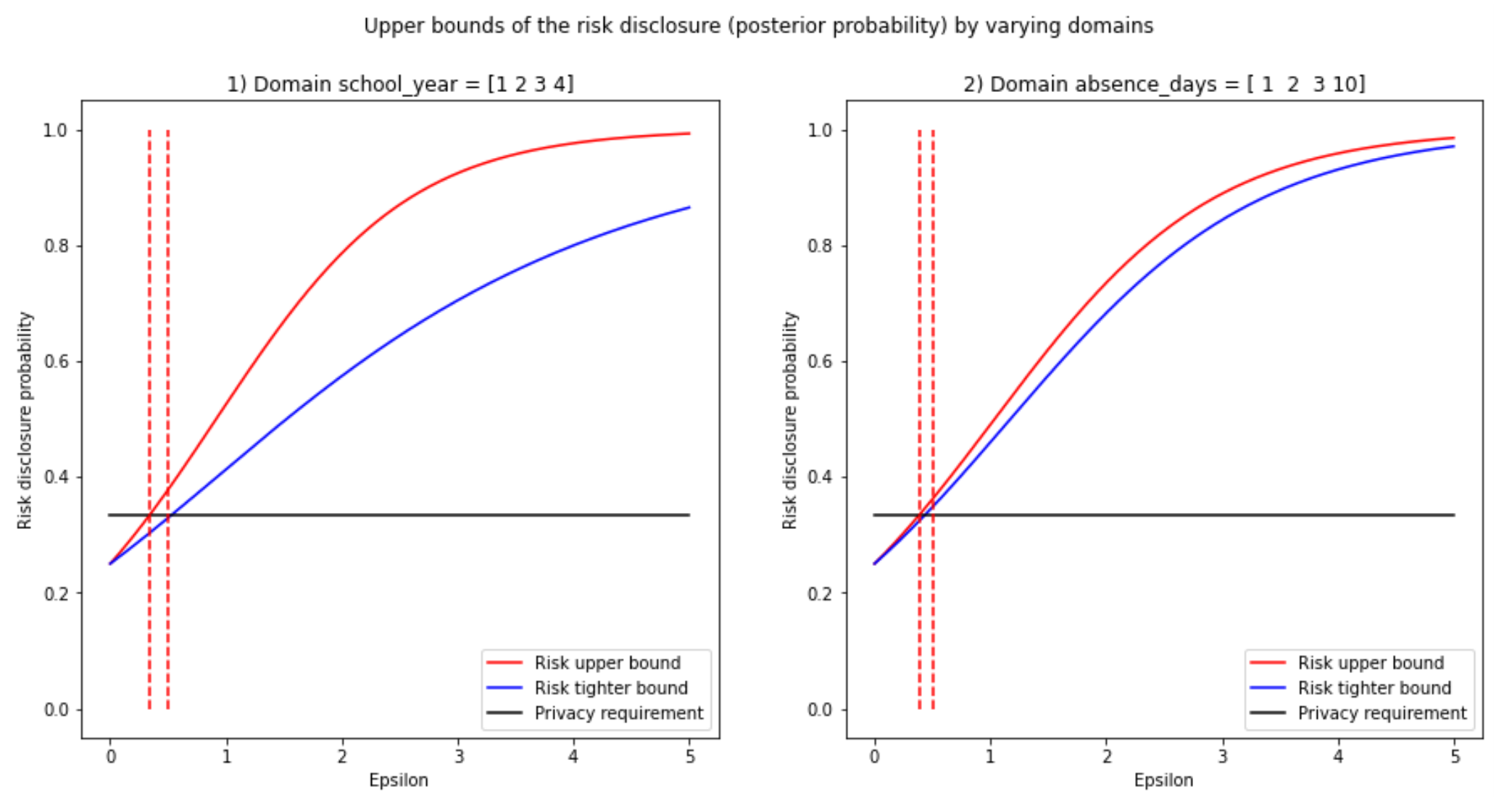
And then we use the classic matplotlib. Note that we have chosen a risk of 1/3 (Black line).
plt.figure(figsize=(15, 7))

risk = 1/3
# Calculate upper bound
epsilon_upper_bound = upper_bound_epsilon(df_school, columns, mean_bounded_global_sensitivities, mean_unbounded_global_sensitivities, risk)

for index, column in enumerate(columns):

    # Start the plot
    plot_index = int(str(1) + str(len(columns)) + str(index+1))
    plt.subplot(plot_index)

    # plot the upper bounds
    upper_bound, = plt.plot(epsilons, posterior_upper_bound[column], 'r',  label="Risk upper bound")
    tighter_bound, = plt.plot(epsilons, posterior_tighter_upper_bound[column], 'b',  label="Risk tighter bound")

    # Plot the risk
    privacy_requirement, = plt.plot(epsilons, np.full(shape=len(epsilons), fill_value=risk), color='black',  label="Privacy requirement")

    # Plot the epsilon upper bound
    y_axis_points = np.linspace(0,1,2)
    plt.plot(np.full(shape=len(y_axis_points), fill_value=epsilon_upper_bound[column]), y_axis_points, 'r--')
    plt.plot(np.full(shape=len(y_axis_points), fill_value=0.5), y_axis_points, 'r--')

    # Legends
    legend = plt.legend(handles=[upper_bound, tighter_bound, privacy_requirement], loc='lower right')

    # axis labels and titles
    plt.xlabel('Epsilon')
    plt.ylabel('Risk disclosure probability')
    plt.title('{}) Domain {} = {}'.format(index+1, column, df_school[column].values))

    # Zoom
#     plt.ylim(0, 0.4)
#     plt.xlim(0, 0.6)

    # Additonal info
    print('Epsilon upper bound for risk {} in universe {} = {}'.format(round(risk, 2), column, epsilon_upper_bound[column]))


plt.suptitle('Upper bounds of the risk disclosure (posterior probability) by varying domains')
plt.show()
>>> Epsilon upper bound for risk 0.33 in universe school_year = 0.3378875900901369
>>> Epsilon upper bound for risk 0.33 in universe absence_days = 0.38293926876882173

You may see that by using the tighter upper bound (Blue) instead of the other bound (Red), you get a better value of epsilon (Larger, which means less noise for the same amount of risk). However, You may appreciate that the red vertical bars are still not optimized (They need to intersect at the crossing between the black line and the two curves).
More specifically: (Looking at plot 1, left plot) The authors want us to notice that even though we have an epsilon bound on 0.3379 (left red dotted vertical line), we can find a higher value of epsilon that still fulfills the privacy requirement (risk disclosure <1/3). E.g., epsilon = 0.5, which corresponds to the right dashed red line, is still to the left of the intersection between the blue and black curves. But note than an epsilon of 0.5 on the absence days plot would make the risk go above the set threshold of 1/3, i.e., the right red dashed line is to the right of the intersection of the black and blue curve.
You cannot free epsilon on one side of the inequality from the tighter bound formula due to arithmetic constraints. Thus, you cannot find epsilon directly on the tighter bound curve formula, unlike with the upper bound curve. Therefore, they propose to use binary search starting at the max of the domain; in this case, it is with an epsilon of 5, which would approximately yield a 100% probability of the adversary being successful.
I also coded a binary search function to find the right values of epsilon (Function in the notebook). Here we call this function directly:
privacy_requirement = 1/3
query_type = 'mean'
posterior_bound_type = 'tight'
columns = ['school_year', 'absence_days']
optimal_epsilons = binary_search_epsilon(df_school, df_school_release, columns, query_type, mean_bounded_global_sensitivities, mean_unbounded_global_sensitivities, privacy_requirement, posterior_bound_type)
print('Optimal epsilons:')
optimal_epsilons
>>> {'school_year': 0.3378877996541445, 'absence_days': 0.3829395062746971}
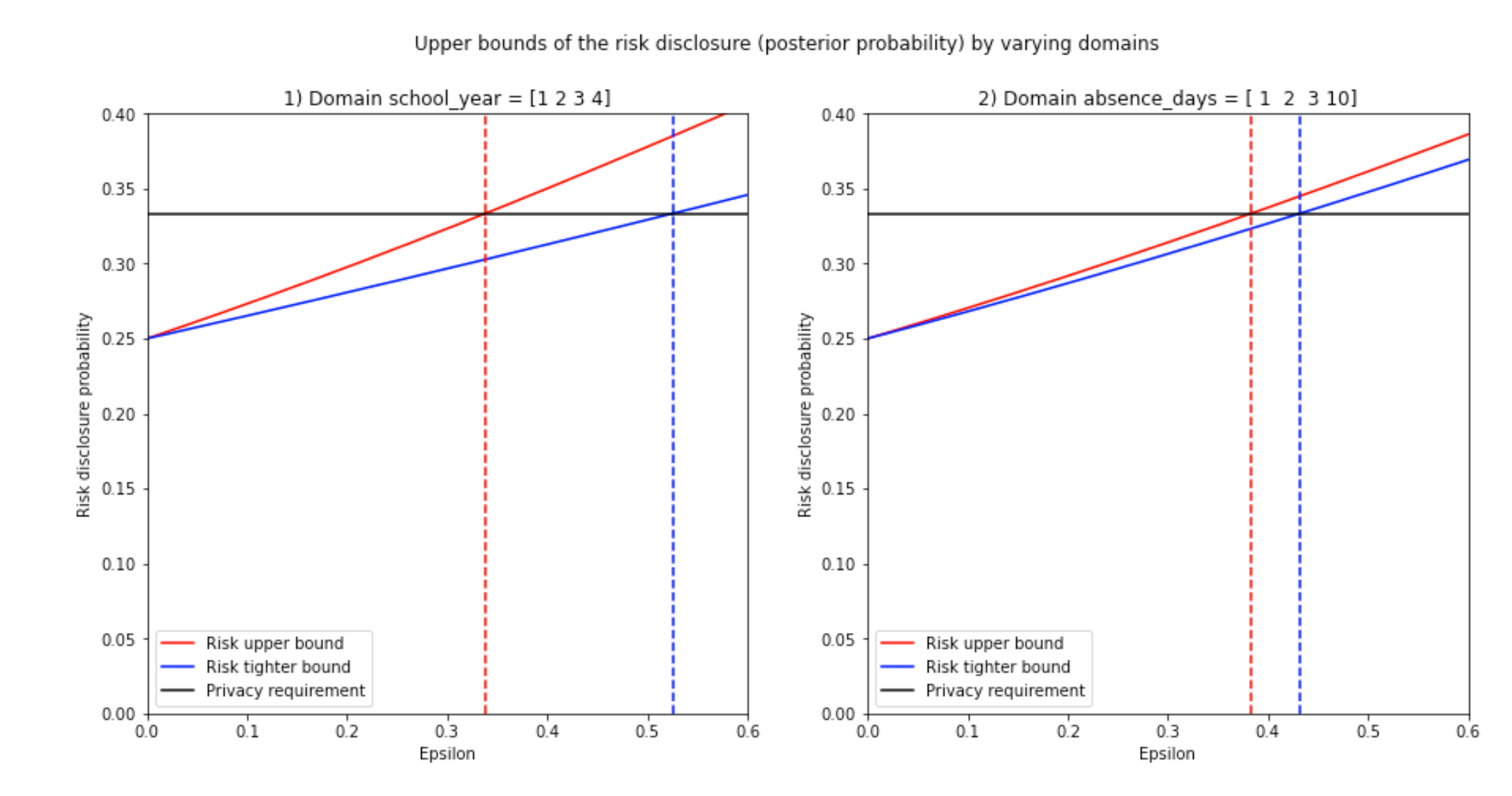
... Some other cells... including plotting..

>>> Plot: 0 school_year
Epsilon upper bound for risk 0.33 in universe school_year = 0.3378875900901369 in dash red
Epsilon tight upper bound for risk 0.33 in universe school_year = 0.525149770057615 in dash blue
>>> Plot: 1 absence_days
Epsilon upper bound for risk 0.33 in universe absence_days = 0.38293926876882173 in dash red
Epsilon tight upper bound for risk 0.33 in universe absence_days = 0.43171996782769506 in dash blue
The optimal epsilons (On dashed blue lines) fit pretty well, they maximize utility while preserving privacy.
The epsilon value for the red-dashed line may be calculated with the formula of the upper bound, but the epsilon value of the blue-dashed line can only be calculated with a binary search using the tighter bound formula.
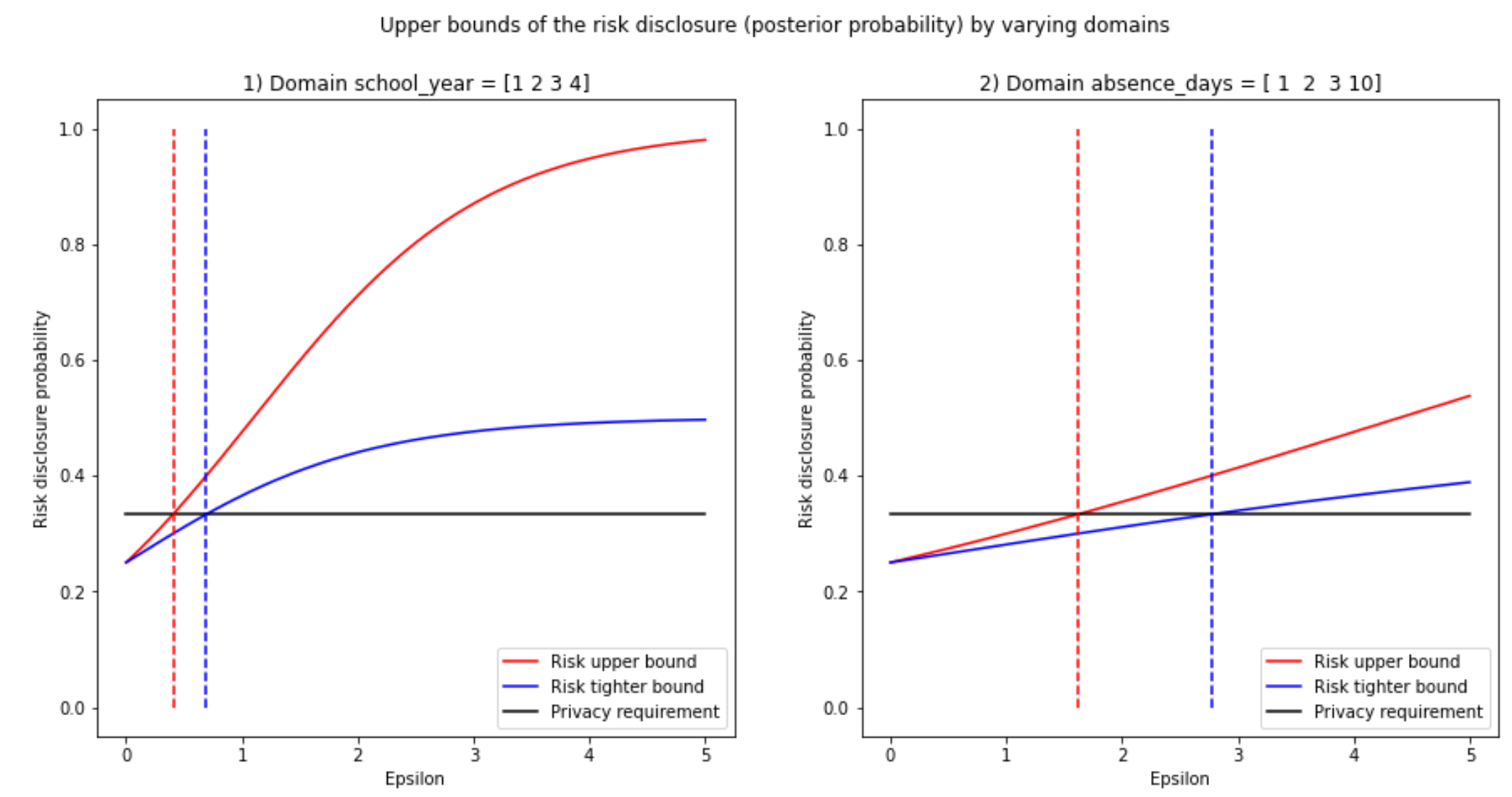
I went ahead and performed the same calculations but for the median query. I invite you to do the same with other queries I programmed in the notebook. Here is the result if we use the median instead:

Clearly, it is worth performing the binary search, as sometimes the bounds diverge more. The divergence of the bounds depends on the dataset and the type of query.
In summary, the authors proposed bounds for epsilon so that its value may not yield a random output query result that leads to a posterior that is greater than the disclosure risk.
I hope you enjoyed the code tutorial! There are more functions and more results replicated in the Notebook.
THE END